Autor da secção: Laiton Hedley

Common Data Recipes

This section provides common data recipes for handling and transforming data in jamovi, such as excluding outliers, reverse scoring survey items, recoding continuous variables to categories, and more.

Excluding Outliers (IQR)

Two common approaches for identifying and removing outliers are the IQR method and the z-score method.

For the IQR method, values that are greater than 1.5 times the interquartile range (IQR) above the third quartile or below the first quartile are considered outliers (of course more strict or lenient thresholds can be applied). Any values outside this range should be filtered out of an analysis, see here for more info.

For example, the data below has two columns one for Memory Score Performance and another for the Absolute IQR of the Memory Score Performance variable. The last two rows of the data show extreme outlier values of 15 and 98 for Memory Score Performance, which have Absolute IQR values of 9.05 and 5.05 respectively, indicating that they are outside the whiskers of a boxplot and should be filtered out of analyses.

Table 15 Memory Scores Pre Filtering (ABSIQR) for Outliers

Memory_Score	ABSIQR(Memory_Score)
68	0
66	0
70	0
…	…
15	9.05
98	5.05

To exclude these outliers from analyses, a filter can be created using the ABSIQR() function in the filter expression: ABSIQR(Memory_Score)<1.5

This filter will include only those rows where the Absolute IQR value is less than 1.5 and thererfore exclude the outliers greater than or equal to 1.5:

Table 16 Memory Scores Post Filtering (ABSIQR) for Outliers

Filter 1	Memory_Score	ABSIQR(Memory_Score)
✔	68	0
✔	66	0
✔	70	0
✔	…	…
✘	15	9.05
✘	98	5.05

As shown above, the filter has excluded the two outliers (15 and 98) with an additional column with crosses to indicate exclusion (excluded rows will also appear as grey/transparent in the data view). Only the non-outlier values (68, 66, 70, etc.) are included in analyses and visualisations, as indicated by ticks in the first column above.

Excluding Outliers (z-score)

For the z-score method, often values that have a z-score +/- 3 are considered outliers and removed for analyses (more lenient or strict thresholds can be applied).

For example, below is a data set with a column for Memory Score Performance and another for the Absolute z-score of the Memory Score Performance variable.

Table 17 Memory Scores Pre Filtering (ABSZ) for Outliers

Memory_Score	ABSZ(Memory_Score)
68	1.08
66	0.93
70	1.23
…	…
15	3.01
98	3.43

The last two rows of the data show outlier values of 15 and 98 for Memory Score Performance, which have Absolute z-score values of 3.01 and 3.43 respectively, indicating that they are outliers and should be filtered out of analyses. To exclude the rows with outliers, the following filter can be used: ABSZ(Memory_Score)<3

Table 18 Memory Scores Post Filtering (ABSZ) for Outliers

Filter 1	Memory_Score	ABSZ(Memory_Score)
✔	68	1.08
✔	66	0.93
✔	70	1.23
✔	…	…
✘	15	3.01
✘	98	3.43

As shown above, the filter has excluded the two outliers (15 and 98) with an additional column with crosses to indicate exclusion (excluded rows will also appear as grey/transparent in the data view). Only the non-outlier values (68, 66, 70, etc.) are included in analyses and visualisations, as indicated by ticks in the first column above.

Reverse Scoring Survey Items

When handling survery data, it is common to have some items that are reverse scored. A simple rule of thumb for reverse scoring is to subtract the item score from the maximum possible score plus one.

For example, below is a table of data in which participants have responded on a 1-7 Likert scale to three items (Item_1, Item_2, and Item_3) that are intended to measure the same construct, but Item_3 is scored such that higher scores indicate less of the construct being measured.

Table 19 Data Pre-Reverse Scoring Survey Item

Item_1	Item_2	Item_3
4	3	3
3	4	5
4	4	2

To reverse score Item_3, click a new column and choose New Computed Variable and use the following: 8 - Item_3 Alternatively, if reverse scoring needs to be applied to multiple items, click a new column and choose New Transformed Variable, choose the item to be reverse score in the Source variable box. Next click, using transformation and choose Create New Transform… and use the following formula: 8 - $SOURCE

Table 20 Data Post-Reverse Scoring Survey Item

Item_1	Item_2	Item_3	Item_3_Reverse_Scored
4	3	3	4
3	4	6	1
4	4	2	5

Once applied the new column (Item_3_Reverse_Scored) will contain the reverse scored values (of Item_3), values of 1 become 7, values of 2 become 6, values of 3 become 5, and so on. Now higher scores on Item_3_Reverse_Scored indicate more of the construct being measured and lower scores indicate less of the construct being measured, which is consistent with the scoring of Item_1 and Item_2. This is a particularly important step to ensure that all items are scored in the same direction before computing a sum score or mean score across items, otherwise the resulting overall score may not accurately reflect the construct being measured.

Attention Checks with a Reverse Scored Item

Often two items in a survery that ask a similar question but are worded in opposite directions, one is reverse worded and the other is not, can be used as an attention check by comparing responses on both. Participants who fail to respond in a consistent way to these two items are likely not paying attention or responding in a biased way (e.g., acquiescent response bias, random response bias).

For example, Item 1: “I never doubt my abilities.” and Item 2: “I often doubt my abilities.” should result in participants responding in a consistent way (i.e., if they strongly agree (5) with Item 1, they should also strongly disagree (1) with Item 2):

Table 21 Attention Check with Reverse Scoring Step 1.

Item_1	Item_2	Item_2_Reverse_Scored
5	1	5
1	5	1
1	2	3

To check if participants are consistently responding to the two items, take the reverse scored version of Item_2 (Item_2_Reverse_Scored) and compare it to Item_1, the absolute difference between should be 0 if participants are responding in a consistent way, and any value greater than 0 indicates inconsistency in responses between the two items.

To do this, first reverse score the item that is reverse worded (in this case Item_2) using the same method as described in the previous section.

Next, in a blank column click New Computed Variable and use the following formula to compute the absolute difference between Item_1 and Item_2_Reverse_Scored: ABS(Item_1 - Item_2_Reverse_Scored)

Table 22 Attention Check with Reverse Scoring Step 2.

Item_1	Item_2	Item_2_Reverse_Scored	Absolute_Difference
5	1	5	0
1	5	1	0
1	2	3	2

Then under the data tab click Filter, here we can filter out paticipants who have an absolute difference greater than 0 by using the following filter expression: Absolute_Difference == 0

Table 23 Attention Check with Reverse Scoring Step 3.

Filter 1	Item_1	Item_2	Item_2_Reverse_Scored	Absolute_Difference
✔	5	1	5	0
✔	1	5	1	0
✘	…	…	…	…

Any participants who did not respond consistenly are now removed and any only participants who responded in a consistent way to the attention check items are included in analyses and visualisations.

Attention Checks with a Single Item

Often a particular item can be used as an attention check, it may say «Please select ‘strongly disagree’ for this item». These items are designed to catch participants who are not paying attention or responding in a biased way (e.g., acquiescent response bias, random response bias). This is an impossible item to fail if participants are truly paying attention.

Below are responses to several items of a survey, where item nine (Item_9_Attention_Check) is an attention check item that instructs participants to select “5” (or strongly agree) to indicate they are paying attention (from a possible 1-5 likert scale):

Table 24 Data Pre-Removing Response Bias Participants

ID	Item_1	Item_2	Item_9_Attention_Check
1	3	3	5
2	5	4	5
3	4	4	4

The last participant (ID 3) has failed the attention check by selecting Agree (“4”) instead of Strongly Agree (“5”) on the attention check item.

In jamovi, to remove participants who fail the attention check, click on Filters near the filter icon and use the following filter expression: Item_9_Attention_Check == 5

Table 25 Data Pre-Removing Response Bias Participants

Filter 1	ID	Item_1	Item_2	Item_9_Attention_Check
✔	1	3	3	5
✔	2	5	4	5
✘	…	…	…	…

Now, only the participants who have passed the attention check are included and any participants who failed the attention check are removed.

Summation (or Total) Score of Survey Items

Sum scores are often computed across multiple items of survey responses to create an overall score for a construct being measured, often to correlate with other variables or compare between conditions. For example, personality questionnaires use multiple items to measure a single personality trait - such as Extraversion. By computing a sum score across those survey items, an overall score (in this case Extraversion Score) can be created for each participant (see here for more info on personality scales).

Below is a table of responses to several items of the subscale of Extraversion, where each item is scored on a 1-5 Likert scale:

Table 26 Data Pre-Summation of Extraversion Items

Item_1	Item_6	Item_11	Item_16
5	1	3	3
4	2	1	1
4	2	4	5

To compute a sum score across these items, click a new column and choose New Computed Variable. By using the SUM() function and choosing the variables (or rather items) of interest, the following formula can be used to compute the sum score: SUM(Item_1, Item_6, Item_11, Item_16)

Table 27 Data Post-Summation of Extraversion Items

Item_1	Item_6	Item_11	Item_16	Extraversion_Sum_Score
5	1	3	3	12
4	2	1	1	8
4	2	4	5	15

As shown above, the new column (Extraversion_Sum_Score) contains the sum score across the items (of Extraversion) with each row indicating the overall score for each participant. This sum score can now be used in analyses and visualisations to correlate with other variables or compare between conditions.

Recoding a Continuous Variable to Categories

Often continuous variables are recoded into categories to create groups for comparison. Age is a common example of a continuous variable that is often recoded into categories such as Young Adults (18-29), Middle-Aged Adults (30-59), and Older Adults (60+). Below is an example of a data set with a column for Age:

Table 28 Data Pre-Recoding Age to Categories

Age
25
18
20
35
30
45
65
62
71

To recode a continuous variable, like age, into categories click on a new column and choose New Transformed Variable. Next, choose the source variable to be the variable of interest (i.e. Age) and click on Using transformation and choose Create New Transform…:

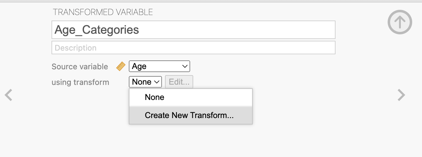
Then click Add recode condition next to the blue plus sign and use the following cutoffs to recode Age into categories:

|ts_recode_age_thresholds|

In the transformation editor, you can set up the recoding logic using conditions such as:

• If Age < 30, then assign «Young»

• If Age < 50, then assign «Middle-Aged»

• Else, assign «Older»

This works because the conditions are evaluated in order. For example:

• Any value less than 30 will be assigned «Young» (so ages 18–29).

• For values not less than 30, the next condition is checked: if Age < 50, assign «Middle-Aged» (so ages 30–49).

• Any value not meeting the previous conditions (i.e., 50 and above) will be assigned «Older» by the final else statement.

This approach allows you to create non-overlapping, ordered Age categories using simple less-than conditions and a final catch-all else.

A new column will appear next to the data, with the recoded categories of Age (Young, Middle-Aged, and Older) based on the cutoffs specified in the transformation:

Table 29 Data Post-Recoding Age to Categories

Age	Age_Categories
25	Young
18	Young
20	Young
35	Middle-Aged
30	Middle-Aged
45	Middle-Aged
65	Older
62	Older
71	Older

This new categorical variable can now be used in analyses and visualisations to compare between Age groups.

Recoding/Reducing the Number of Categories

Often categorical variables have many categories, and it can be useful to recode or reduce the number of categories for more simple analysis or visualisation. Smoker status is a common example of this, smoker status could be either; Non-smoker, Occasional Smoker, Regular Smoker, or Heavy Smoker:

Table 30 Data Pre-Reducing Smoker Status to Categories

Smoker_Status
Non-smoker
Occasional Smoker
Regular Smoker
Heavy Smoker

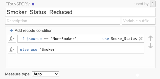
Reducing these categories to two, Non-smoker and Smoker, can be useful for simple comparisons between Smokers and Non-smokers. To reduce the number of categories, click on a new column and choose New Transformed Variable. Next, choose the source variable to be the variable of interest (i.e. Smoker_Status) and click on Using transformation and choose Create New Transform….

Non-smokers can be left as is, while the other categories can be combined into a single «Smoker» category. The following recoding logic can be applied to reduce the number of categories:

A new column will appear next to the data, with the recoded categories of Smoker Status (Non-smoker and Smoker):

Table 31 Data Post-Reducing Smoker Status to Categories

Smoker_Status	Smoker_Status_Reduced
Non-smoker	Non-smoker
Occasional Smoker	Smoker
Regular Smoker	Smoker
Heavy Smoker	Smoker

The new column of data, Smoker_Status_Reduced, can now be used in analyses and visualisations to compare between Smokers and Non-smokers.

Restricting Analyses to a Subset of Data

At times only a subset of data is needed for an analysis, it may be useful to restrict the data to a subset of interest. In jamovi to restrict any analyses to a single group this is as simple as applying a Filter.

A Filter can be used to restrict the data to only the rows of interest - which is best used if the other subset of data is of no interest and can be excluded from all analyses (see the following section if interested in keeping subsets and splitting output via categories).

Below is an example of a data set with three variables, Region, Education Level, and Total Survey Score:

Table 32 Data Pre-Filtering to Analyse a Subset of Data

Region	Education Level	Total Survey Score
North America	High School	15
North America	University	20
Europe	High School	10
Europe	University	25
North America	High School	12
Europe	University	22

Perhaps there is interest in comparing the Total Survey Score of participants between Education Levels, but only for participants from North America (and exclude any from Europe).

To do so, a filter (option 2) to the overall data set is best suited, click on the data tab and select Filters under the filter icon, then use the following expression: Region == 'North America'

Table 33 Data Post-Filtering to Analyse a Subset of Data (Option 2)

Filter 1	Region	Education Level	Total Survey Score
✔	North America	High School	15
✔	North America	University	20
✘	…	…	…
✘	…	…	…
✔	North America	High School	12
✘	…	…	…

A new column will appear with ticks to indicate which rows are included and crosses to indicate which rows are excluded. jamovi will now only consider participants from North America (or rather rows with ticks) for any analyses and visualisations.

Anlaysing Subsets of Data (AKA Split File)

It can be useful to analyse two or more subsets of data separately, this is often referred to as a Split File in other statistical software.

Below is an example of a data set with three variables, Region, Education Level, and Total Survey Score.

Table 34 Data Pre-Filtering to Analyse a Subset of Data

Region	Education Level	Total Survey Score
North America	High School	15
North America	University	20
Europe	High School	10
Europe	University	25
North America	High School	12
Europe	University	22

Perhaps there is interest in comparing the Total Survey Score of participants between Education Levels, but want to analyse or rather split output via geographical location North America and Europe separately. Such data handling can be achieved in jamovi, although currently there is a lack of simple functionality to split the output of analyses by a category and requires a somewhat round about approach to achieve this.

To begin, two New Computed Variables need to be created. The first must filter to only include participants from North America. To do this, click on a new column and choose New Computed Variable, give it a name (e.g., Total_Survey_Score_NorthAm) and use the following formula: FILTER(`Total Survey Score`, Region == 'North America')

The new data column (Total_Survey_Score_NorthAm`) contains Total Survey Scores only for participants from North America, with missing values assigned to participants from other countries, allowing it to be used in analyses and visualisations comparing Education Levels among North American participants while excluding participants from Europe:

Table 35 Data Mid-Filtering to Analyse Subsets of Data

Region	Education Level	Total Survey Score	Total_Survey_Score_NorthAm
North America	High School	15	15
North America	University	20	20
Europe	High School	10
Europe	University	25
North America	High School	12	12
Europe	University	22

The second New Computed Variable must filter to only include participants from Europe. To do this, click on a new column and choose New Computed Variable, give it a name (e.g., Total_Survey_Score_Europe) and use the following formula: FILTER(`Total Survey Score`, Region == 'Europe')

Table 36 Data Post-Filtering to Analyse Subsets of Data

Region	Education Level	Total Survey Score	Total_Survey_Score_NorthAm	Total_Survey_Score_Europe
North America	High School	15	15
North America	University	20	20
Europe	High School	10		10
Europe	University	25		25
North America	High School	12	12
Europe	University	22		22

Using the new columns of data (Total_Survey_Score_NorthAm and Total_Survey_Score_Europe), the same analyses can be run to compare between Education Levels for participants from North America and Europe separately using the respective columns of data.

String Concatenation

String concatenation is the process of joining two or more strings of text together to create a new string. Categorical variables are often represented as strings of text, and sometimes it can be useful to combine information from multiple categorical variables into a single variable.

For example, here are two variables Condition and Time:

Table 37 Pre-String Concatenation Example

Participant_ID	Condition	Time
1	Control	Pre
1	Control	Post
2	Therapy	Pre
2	Therapy	Post
3	Control	Pre
3	Therapy	Post

Combining the information from both Condition and Time can be a simple way to represent the different conditions and time points in a single variable.

To do this, click on a new column and choose New Computed Variable, give it a name (e.g., Condition_Time) and use the following formula: Condition + '_' + Time

Table 38 Post-String Concatenation Example

Participant_ID	Condition	Time	Condition_Time
1	Control	Pre	Control_Pre
1	Control	Post	Control_Post
2	Therapy	Pre	Therapy_Pre
2	Therapy	Post	Therapy_Post
3	Control	Pre	Control_Pre
3	Therapy	Post	Therapy_Post

The new Condition_Time variable contains the combined information from both Condition and Time, with an underscore used to separate the two pieces of information (note this underscore can be excluded if desired). This new variable can now be used in analyses and visualisations to compare between the different conditions and time points in a more simple way than having to consider both Condition and Time separately.

Date Handling

Date handling in jamovi is currently fairly limited. There is no “native” Date data type at this time (one is planned however). The following describes a number of date manipulations that are available.

There are two useful date functions, DATEVALUE() and DATE(), that can be used with Computed Variables. DATEVALUE() converts a date string such as 2025-01-29 to an integer representing the number of days since January 1st, 1970. DATE() performs the opposite transformation, converting such an integer into a date string. A useful way to use these functions is to first convert the date to an integer, perform some computation, and then convert the result back to a date string. Both functions optionally take a date format string if using a particular format.

Table 39 Example date formatting

Day	DATE(Day)	DATE(Day, "%d %m %Y")	DATE(Day, "%m/%d/%y")
13	1970-01-13	13 01 1970	01/13/81
4197	1981-06-29	29 06 1981	06/29/81

Computing a date in the future

The following example converts a date to an integer, adds 7 (representing 7 days), and then converts it back to a date string.

Table 40 Adding 7 days to a date

Date	DATEVALUE(Date)	DATEVALUE(Date) + 7	DATE(DATEVALUE(Date) + 7)
2026-01-29	20482	20489	2026-02-05
2024-03-10	19792	19799	2024-03-17
2025-08-22	20322	20329	2025-08-29

Computing days elapsed

Table 41 Computing days elapsed

StartDate	EndDate	DATEVALUE(EndDate) - DATEVALUE(StartDate)
2026-01-29	2026-02-15	17
2024-03-10	2024-04-11	32
2025-08-22	2024-04-11	-498

Extracting month, year, or day

The SPLIT() function can be used to extract the year, month, or day of month, from a date string. The SPLIT() function takes a text value (such as a date string), splits it into chunks using the second argument as the delimeter, and returns the nth chunk, determined by the third argument. Note that SPLIT() returns a text value, which will needs to be converted to an integer (with the INT() function) if to be used in arithmetic.

Table 42 Extracting month, year, or day

Date	SPLIT(Date, '-', 1)	SPLIT(Date, '-', 2)	SPLIT(Date, '-', 3)
2026-01-29	2026	01	29
2024-03-10	2024	03	10
2025-08-22	2025	08	22

Composing a date from parts

Table 43 Composing a date from parts

Year	Month	DayOfMonth	Year + '-' + Month + '-' + DayOfMonth
2026	01	29	2026-01-29
2024	03	10	2024-03-10
2025	08	22	2025-08-22