Section author: Rebecca Vederhus, Sebastian Jentschke
From SPSS to jamovi: Linear regression
This comparison shows how a linear model with several predictors is conducted in SPSS and jamovi. The SPSS test follows the description in chapter 9.10 - 9.11 in Field (2017), especially figure 9.15-9.19 and 9.22-9.23 as well as output 9.5-9.12. It uses the data set Album Sales.sav which can be downloaded from the web page accompanying the book.
| SPSS | jamovi |
|---|---|
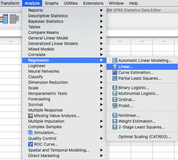
In SPSS, the following steps activates a linear regression: Analyze →
Regression → Linear. |
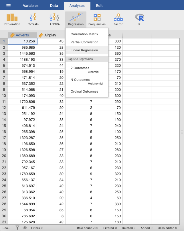
In jamovi, this can be done using: Analyses → Regression → Linear
Regression. |
 |
 |
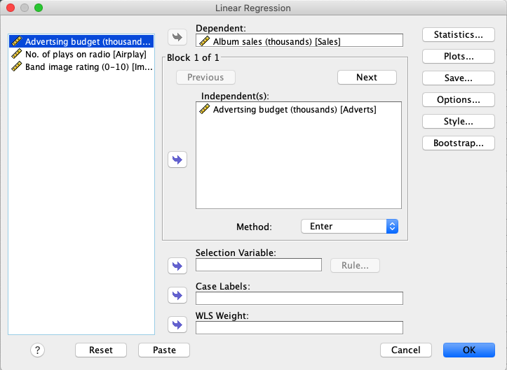
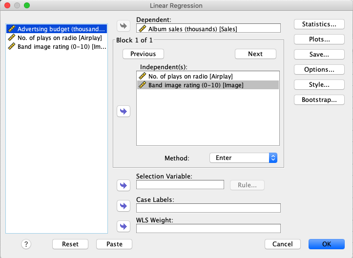
Move the variable Sales to the variable box Dependent and the
variable Adverts to the variable box Independent(s). |
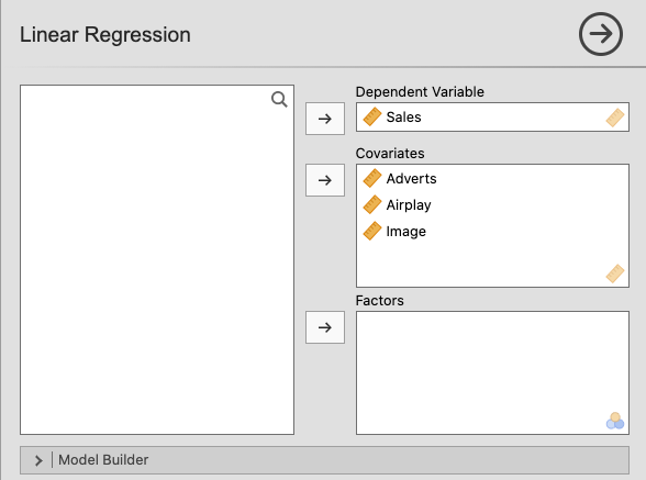
Move Sales to the Dependent Variable box, and the variables
Adverts, Airplay and Image to the box called Covariates. |
 |
 |
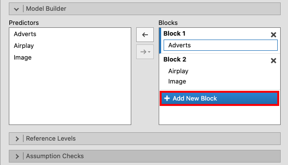
Press Next to create a new block, and add the variables Airplay and
Image to this Independent(s) box. |
In the Model Builder window, create a new block by clicking + Add New
Block and move the variables Airplay and Image to Block 2. |
 |
 |
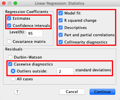
In the Statistics dialog box, select the options shown in the picture
below. |
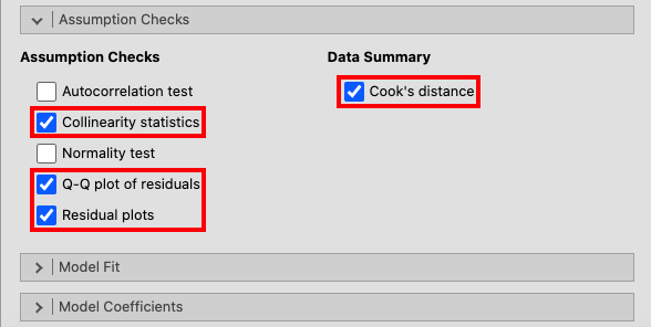
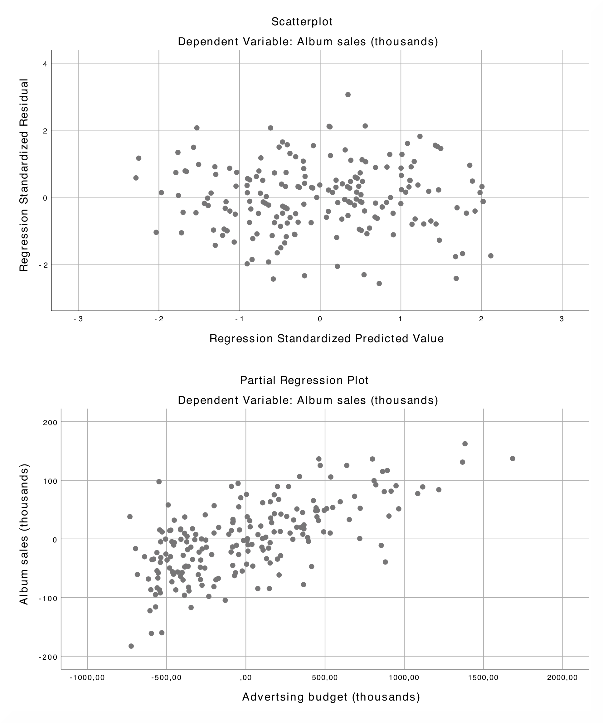
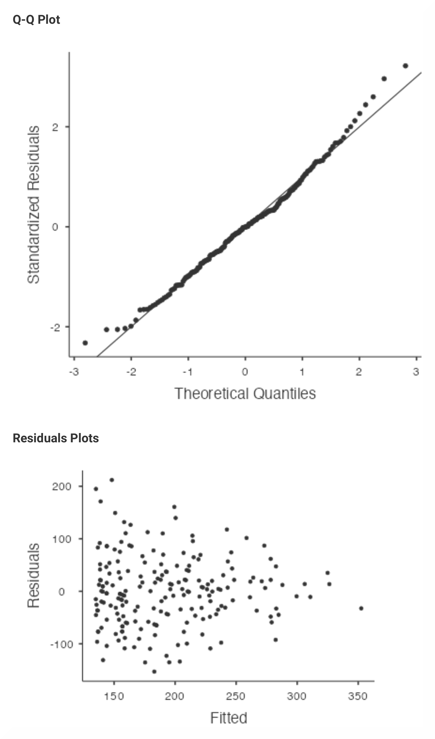
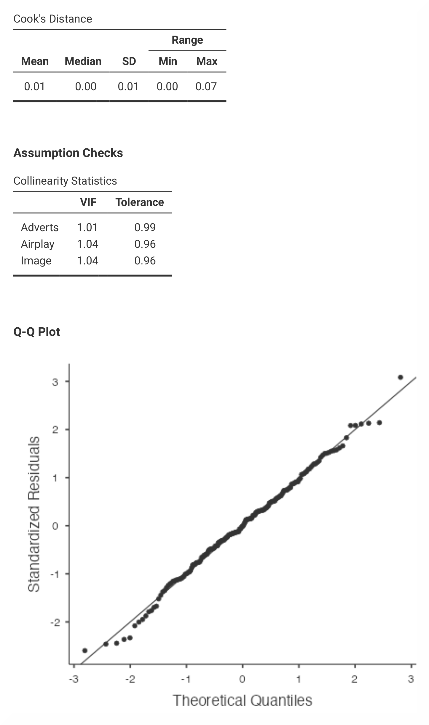
Under Assumption Checks click Collinearity statistics, Q-Q plot of
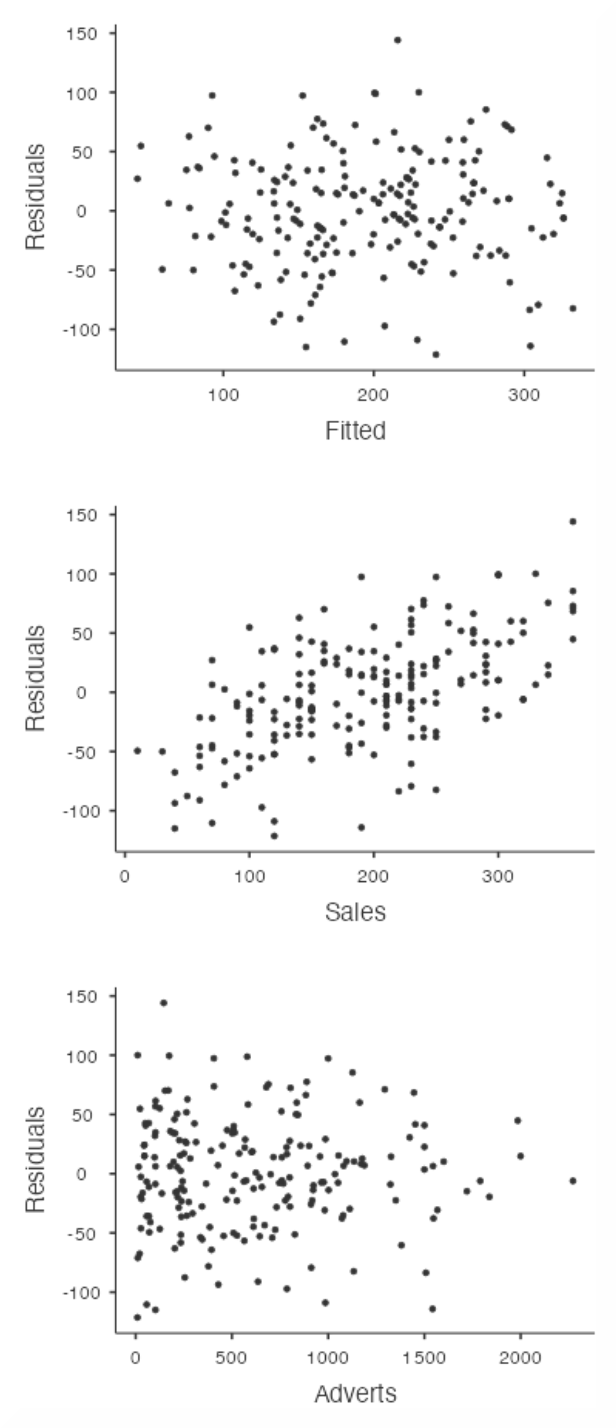
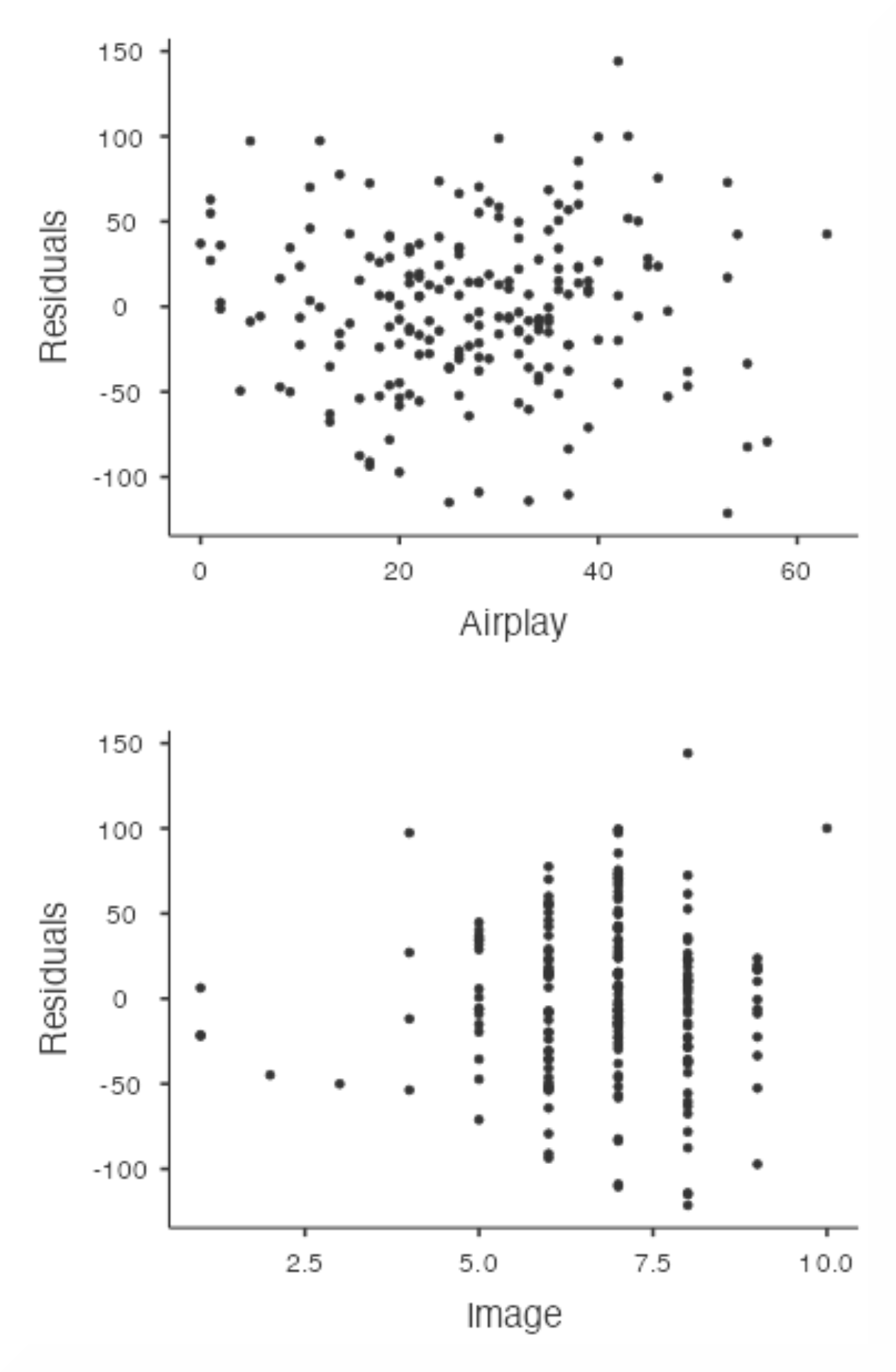
residuals, Residuals plots and Cook’s distance. |
 |
 |
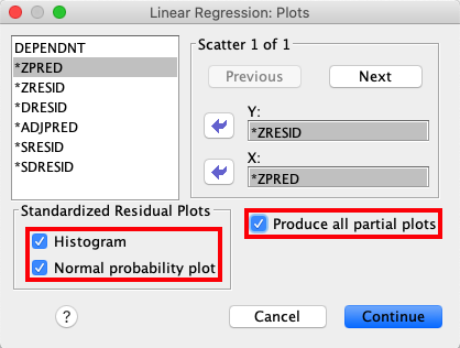
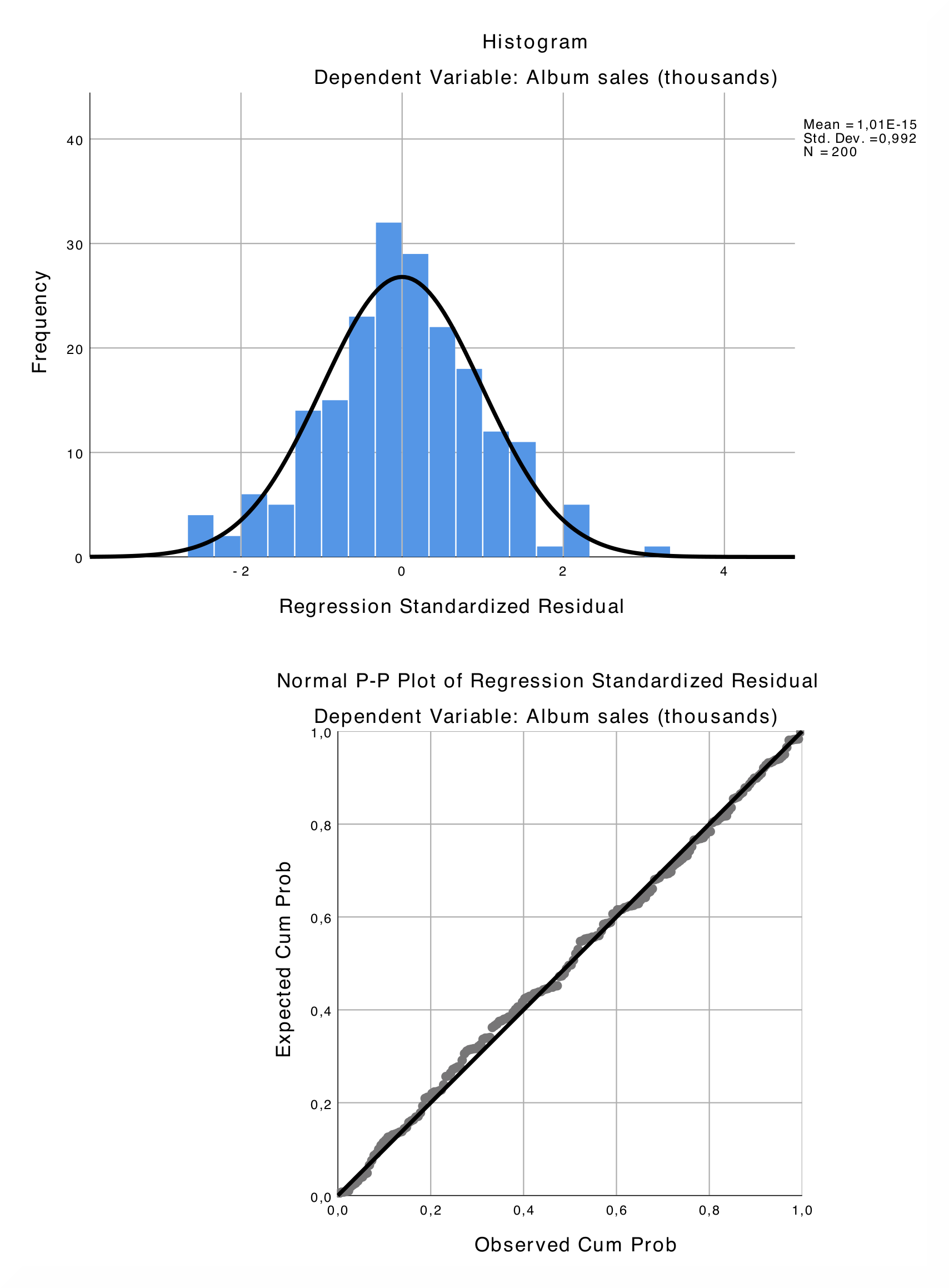
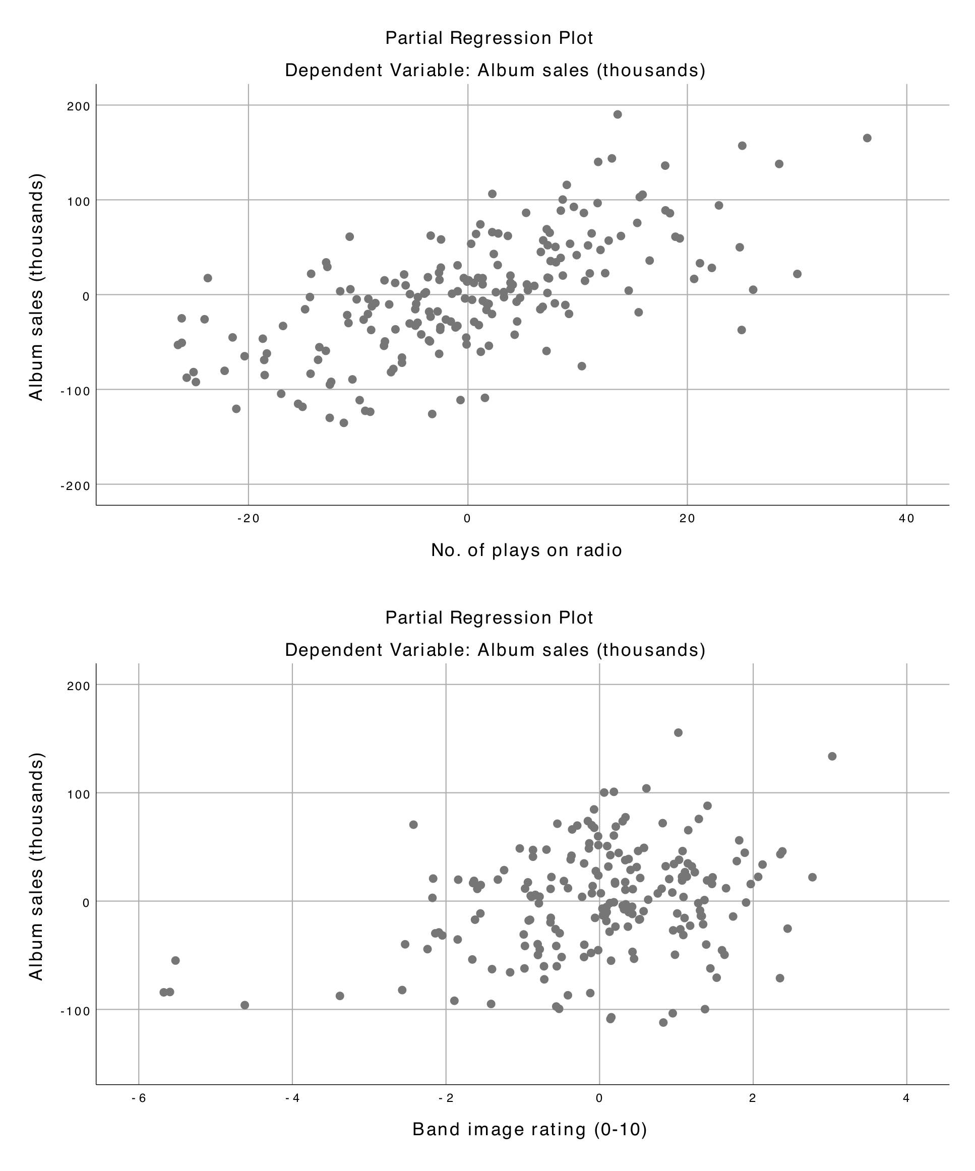
From the main menu, open the Plots window and assign \*ZRESID to the
to the box labelled Y and \*ZPRED to the box labelled X. In
addition, select the options Histogram, Normal probability plot and
Produce all partial plots. |
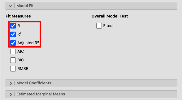
Open the Model Fit window and choose R, R² and Adjusted R². |
 |
 |
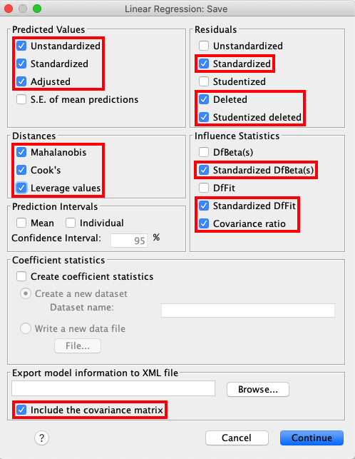
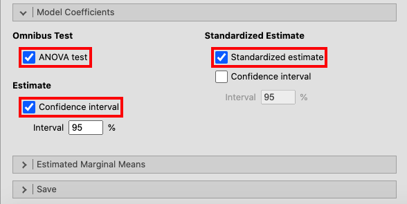
| Open the Save` window from the main menu and select the same options as seen in the picture below. | In the Model Coefficients window, click ANOVA test, Confidence
interval and Standardized estimate. |
 |
 |
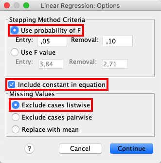
Lastly, activate the dialog box for Options and select Use probability
for F, Include constant in equation and Exclude cases listwise. |
|
 |
|
| The results are essentially the same in SPSS and in jamovi, although they are found in slightly different places. Also, jamovi does not provide all of the information that can be found in the SPSS output. | |
|
|
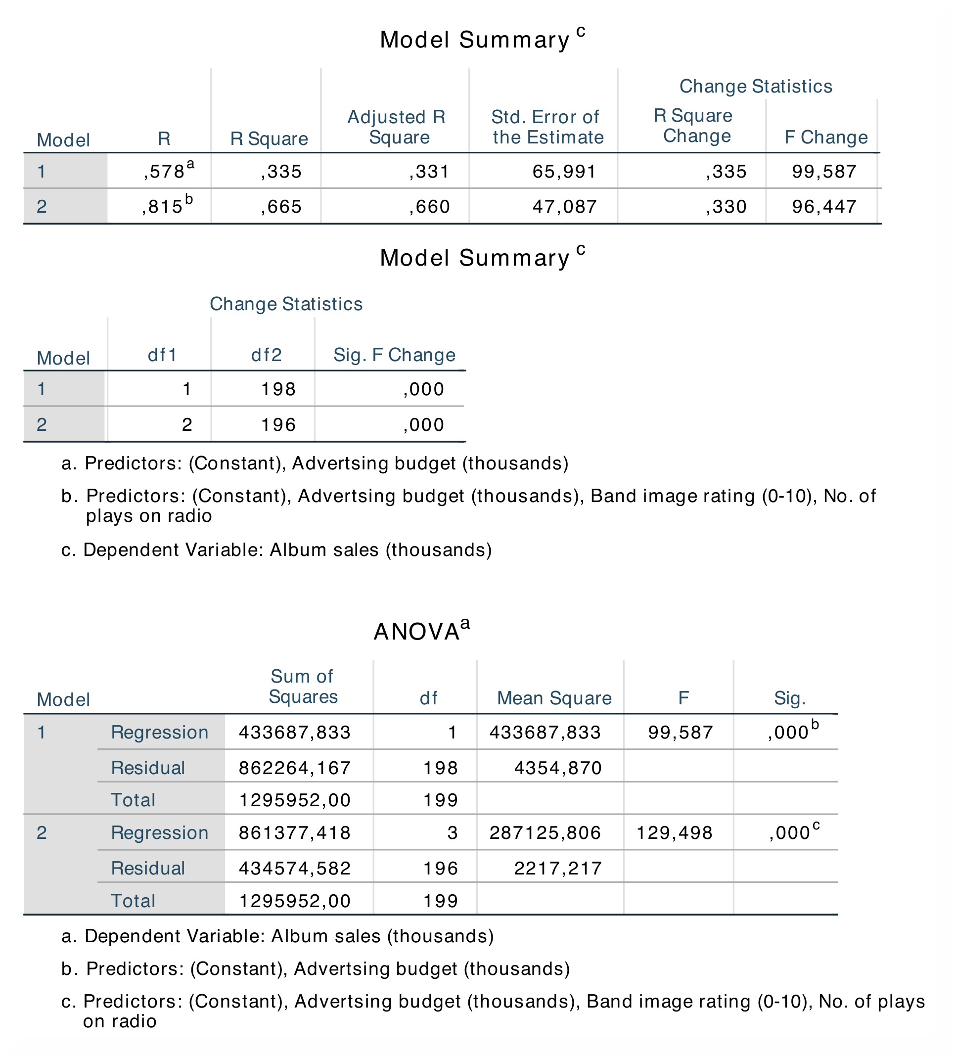
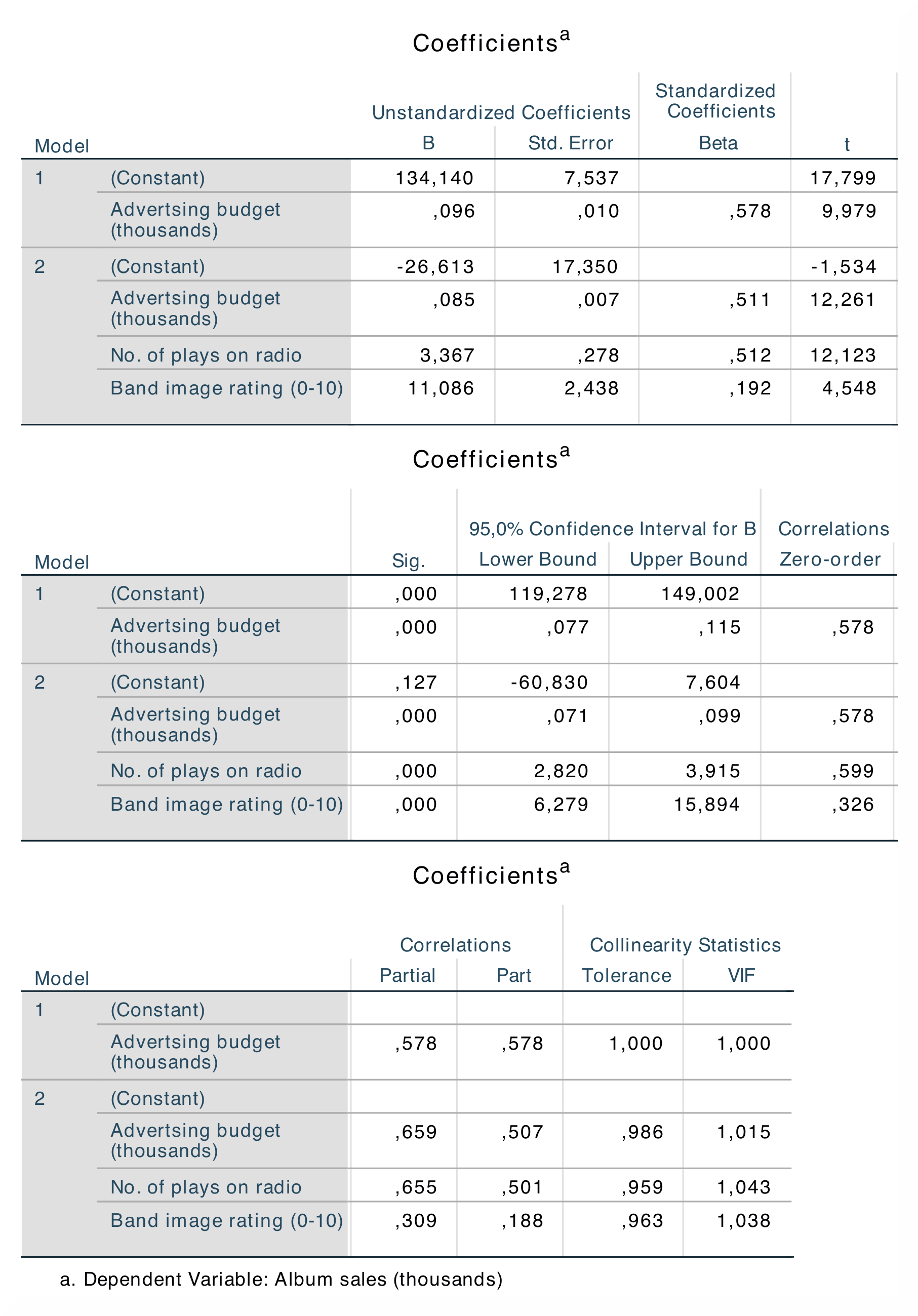
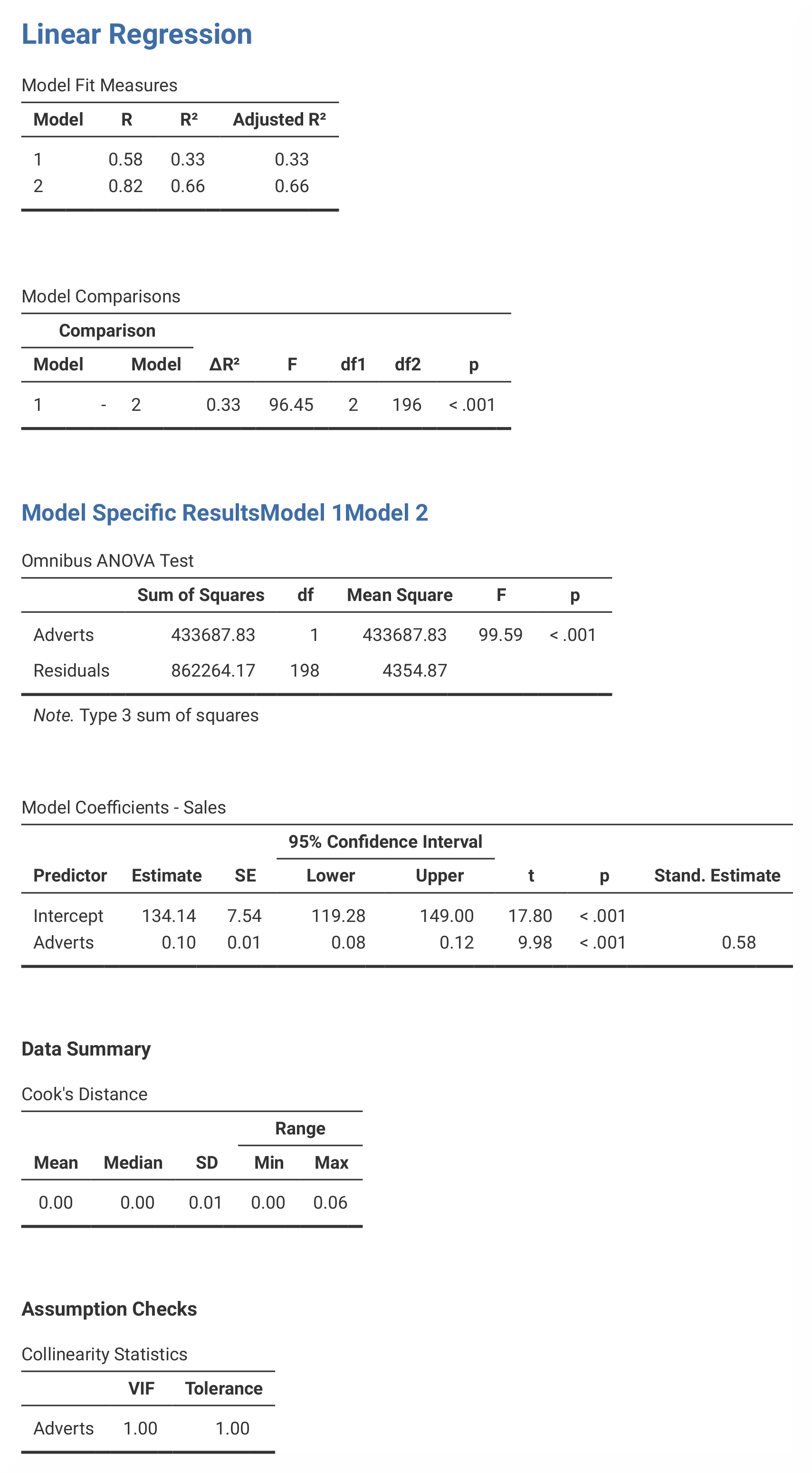
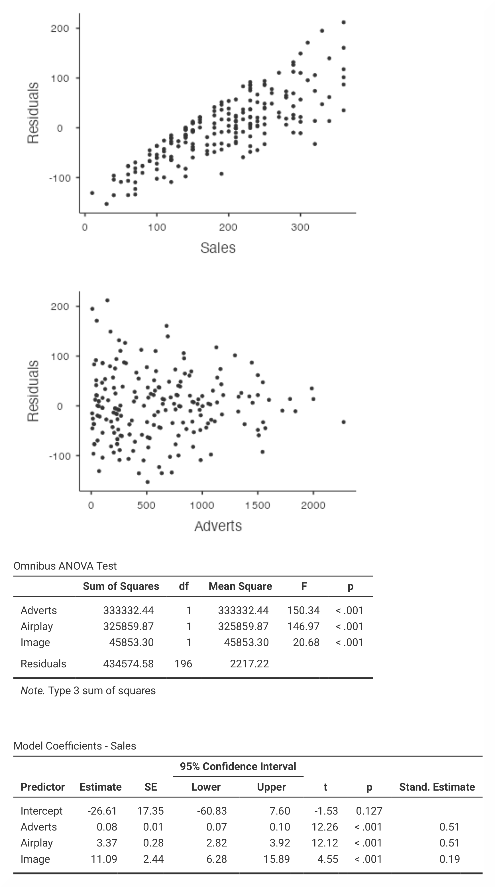
| In the Model Summary, you can see the summary statistics for model 1, where the only predictor is advertising budget, as well as for model 2, in which all three predictors are used. The R²-value of 0.66 in model 2 tells us that advertising budgets, image and airplay together accounts for 66.5% of the variance in album sales. The standardised beta values (β) indicate what happens to the outcome if one predictor changes by one standard deviation. The beta values for all the variables are easily comparable (β = 0.51, β = 0.51 and β = 0.19) because they are almost the same. According to the results, the overall sales will increase by 0.512 standard deviations if the number of radio plays the week before the release date increase by 1 standard deviation (12.27). Significance levels for all beta values are also important to note. | In jamovi, the R²-value is found in the Model Fit Measures table and the beta values are found in the Model Coefficients – Sales table. The ANOVA and Coefficients tables for model 1 and 2 are found in separate tables, whereas in SPSS both models are presented in the same tables. Also, the Model Summary is divided into two different tables in jamovi – Model Fit Measures and Model Comparisons. |
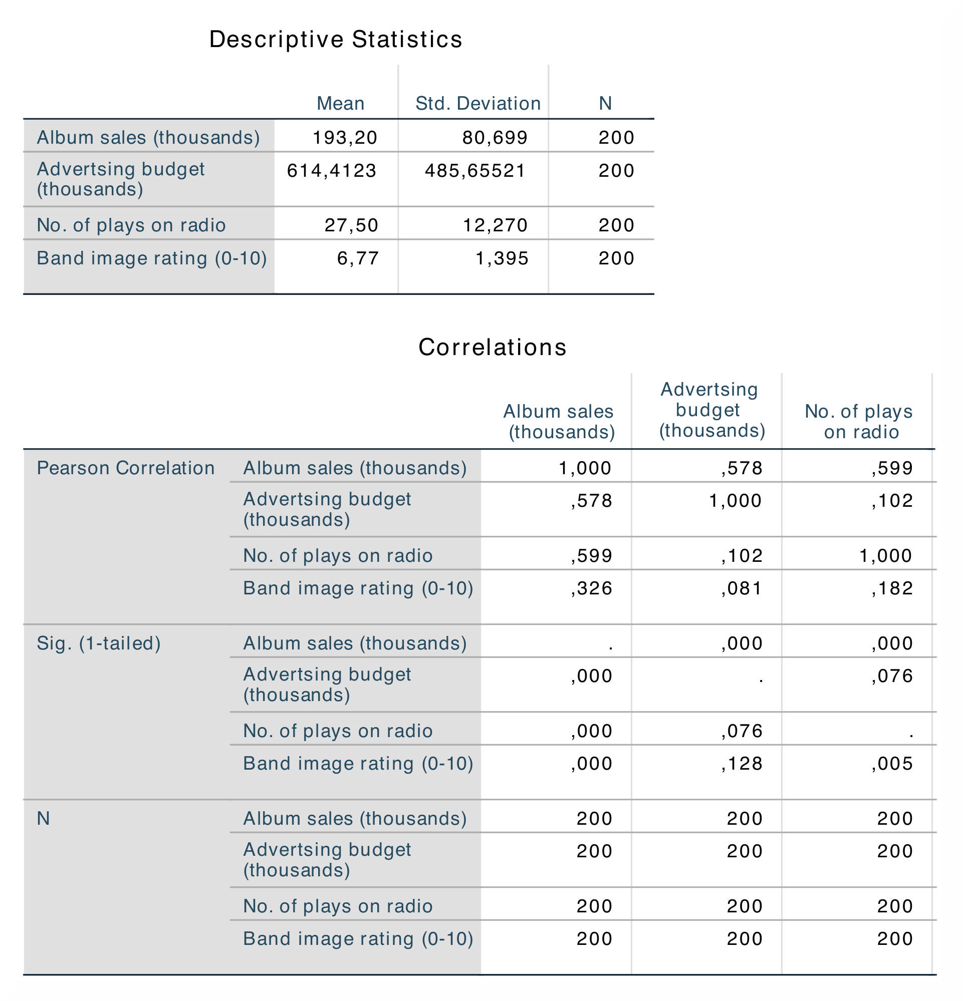
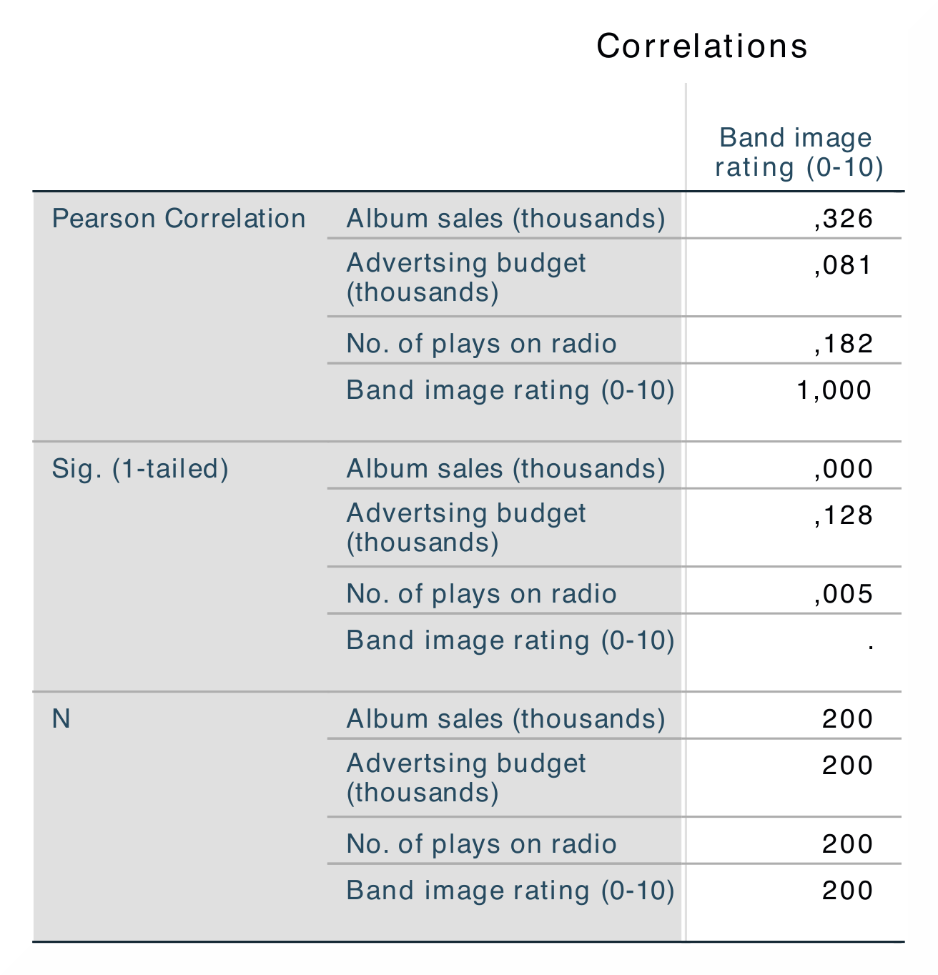
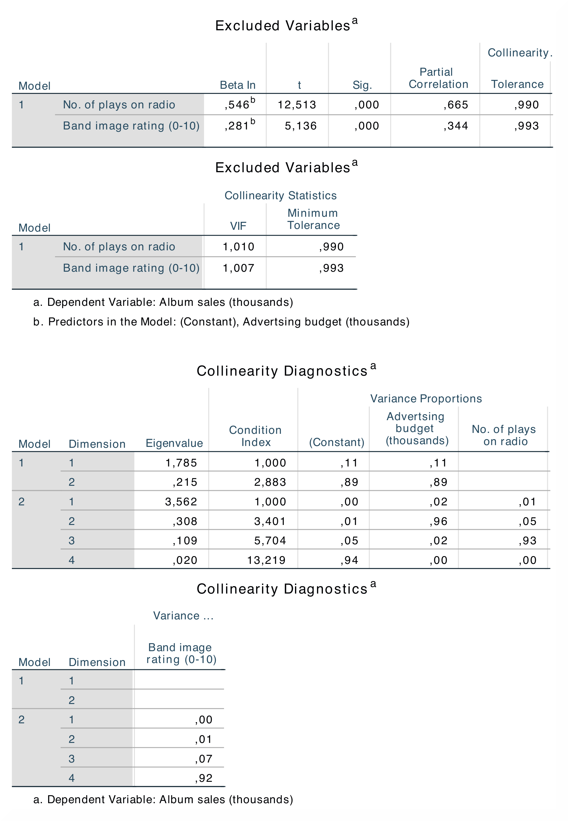
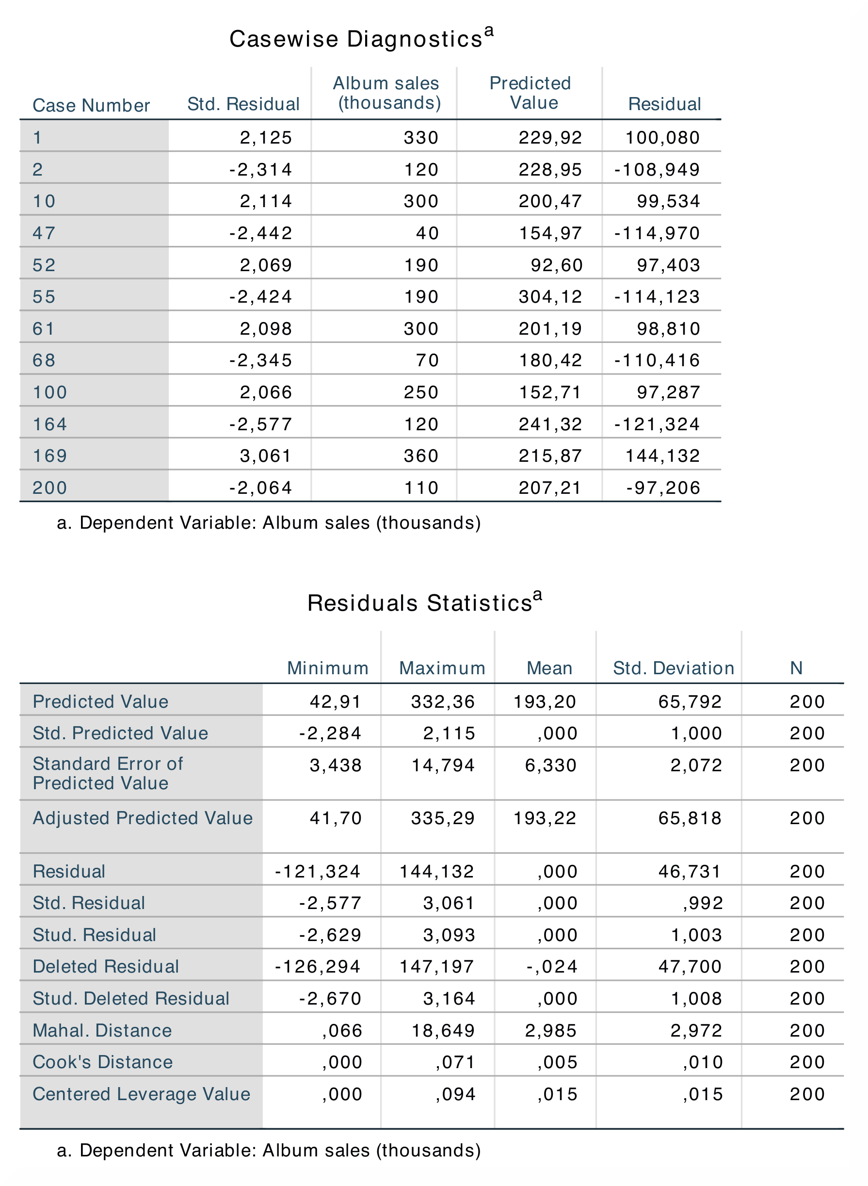
| When doing a linear regression analysis, SPSS produces several output tables that are not produced in jamovi. For instance, jamovi does not provide tables for Descriptive Statistics, Correlations, Casewise Diagnostics and Residuals Statistics. However, jamovi does provide tables for Model Summary, ANOVA and Coefficients, which show the most important findings from the regression. Furthermore, jamovi does not produce an F-statistic for model 2 or a Std. Error of the Estimate. Similar to the analysis on the previous page, the numerical outputs for the current analysis are identical: R = 0.82, R² = 0.66; β = 0.51, p < .001; β = 0.51, p < .001; β = 0.19, p < .001. | |
| If you wish to replicate those analyses using syntax, you can use the commands below (in jamovi, just copy to code below to Rj). Alternatively, you can download the SPSS output files and the jamovi files with the analyses from below the syntax. | |
REGRESSION
  /DESCRIPTIVES MEAN STDDEV CORR SIG N
  /MISSING LISTWISE
  /STATISTICS COEFF OUTS CI(95) R ANOVA COLLIN TOL CHANGE ZPP
  /CRITERIA=PIN(.05) POUT(.10)
  /NOORIGIN
  /DEPENDENT Sales
  /METHOD=ENTER Adverts
  /METHOD=ENTER Airplay Image
  /PARTIALPLOT ALL
  /SCATTERPLOT=(\*ZRESID ,\*ZPRED)
  /RESIDUALS HISTOGRAM(ZRESID) NORMPROB(ZRESID)
  /CASEWISE PLOT(ZRESID) OUTLIERS(2)
  /SAVE PRED ZPRED ADJPRED MAHAL COOK LEVER ZRESID DRESID SDRESID SDBETA
     SD FIT COVRATIO.
|
jmv::linReg(
    data = data,
    dep = Sales,
    covs = vars(Adverts, Airplay, Image),
    blocks = list(
        list("Adverts"),
        list("Airplay", "Image")),
    refLevels = list(),
    r2Adj = TRUE,
    anova = TRUE,
    ci = TRUE,
    stdEst = TRUE,
    qqPlot = TRUE,
    resPlots = TRUE,
    collin = TRUE,
    cooks = TRUE)
|
| SPSS output file containing the analyses | jamovi file containing the analyses |
References
Field, A. (2017). Discovering statistics using IBM SPSS statistics (5th ed.). SAGE Publications. https://edge.sagepub.com/field5e