Autor des Abschnitts: Jonathon Love

Die Datentabelle

In jamovi werden die Daten in einer Tabelle dargestellt, in der jede Spalte eine „Variable“ darstellt.

Datenvariablen

Die am häufigsten verwendeten Variablen in jamovi sind „Datenvariablen“. Diese Variablen enthalten Daten, die entweder aus einer Datendatei geladen oder vom Benutzer „eingetippt“ wurden. Datenvariablen können einer der drei folgenden Datentypen sein:

• Integer
• Decimal
• Text

und eines von vier Skalenniveaus:

• Nominal
• Ordinal
• Continuous
• ID

Die Skalenniveaus werden durch das Symbol in der Kopfzeile der Variablenspalte angezeigt. Beachten Sie, dass einige Kombinationen von Datentyp und Skalenniveau nicht als Kombination auftreten können / sollten und das jamovi Sie solche Kombinationen nicht wählen lässt.

Nominal und Ordinal kennzeichnen nominale und ordinale Variablen. Continuous ist für Variablen mit numerischen Werten, die als Intervall- oder Ratio-Skalen betrachtet werden (äquivalent zu Scale in SPSS). Der Skalentyp ID existiert nur in jamovi. Er ist für Variablen gedacht, die Identifikatoren enthalten, die man nie analysieren möchte (z.B. Name oder ID eines Versuchsteilnehmers). Der Vorteil von IDs ist, dass jamovi intern keine Liste von Faktorstufen im Speicher halten muss (R repräsentiert Text-Variablen intern oft als Faktoren), was die Leistung bei der Interaktion mit sehr großen Datensätzen verbessern kann.

Wenn Sie mit einer leeren Datentabelle beginnen und Werte eingeben, ändern sich Datentypen und Skalenniveaus automatisch in Abhängigkeit von den eingegebenen Daten. Dies ist eine gute Möglichkeit, ein Gefühl dafür zu bekommen, welche Variablentypen zu welcher Art von Daten passen. In ähnlicher Weise versucht jamovi beim Öffnen einer Datendatei den am besten passenden Variablentyp aus den Daten in jeder Spalte abzuleiten. In beiden Fällen kann es sein, dass diese automatische Bestimmung nicht korrekt ist. Daher kann es notwendig werden, den Datentyp und das Skalenniveau im Nachhinein manuell anzupassen.

Der Variablen-Editor kann durch Auswahl von Setup auf der Registerkarte Data, durch Doppelklick auf die Spaltenüberschrift der betreffenden Variable oder durch das Drücken von F3 aufgerufen werden. Im Variablen-Editor können Sie den Namen der Variable und (bei Datenvariablen) den Datentyp, das Skalenniveau, die Stufen eines Faktors und das Label / die Bezeichnung für die unterschiedlichen Faktorstufen ändern. Der Variablen-Editor kann durch Anklicken des Schließpfeils oder durch erneutes Drücken der Taste F3 verlassen werden.

Neue Variablen können mit der Schaltfläche Add aus dem Data`-Tab in den Datensatz eingefügt (vor der aktuellen Cursor-Position) oder angehängt werden (am Ende der existierenden Variablen). Die Schaltfläche ``Add ermöglicht auch das Hinzufügen von Berechneten Variablen.

Berechnete Variablen

Berechnete Variablen sind solche, die ihren Wert durch die Durchführung einer Berechnung basiert auf einer oder mehreren anderen Variablen erhalten. Berechnete Variablen können für eine Reihe von Zwecken verwendet werden, z. B. für logarithmische Transformationen, z-Transformationen, das Berechnen von Skalenwerten (Summe oder Mittelwert), für die Inversion von Skalenitems, etc.

Berechnete Variablen können dem Datensatz mit der Schaltfläche Add, die unter der Registerkarte Data verfügbar ist, hinzugefügt werden. Dabei wird ein Formel-Feld angezeigt, in dem Sie die Formel angeben oder zusammenklicken (fx-Button) können. Es stehen die üblichen arithmetischen Operatoren zur Verfügung. Einige Beispiele für Formeln sind:

A + B
LOG10(len)
MEAN(A, B)
(dose - VMEAN(dose)) / VSTDEV(dose)
Z(dose)

In dieser Reihenfolge sind das die Summe von A und B, eine logarithmische Transformation (zur Basis 10) von len, der Mittelwert von A und B, und der z-Score von dose (mit zwei unterschiedlichen Berechnungsmethoden).

Darüber hinaus sind viele weitere Funktionen verfügbar.

V-Funktionen

Von einer Reihe von Funktionen gibt es Paare, wobei dem einen Teil des Paares ein V vorangestellt ist und dem anderen nicht. V-Funktionen führen ihre Berechnung auf einer Variablen als Ganzes durch (spaltenweise), während Funktionen ohne V ihre Berechnung zeilenweise durchführen. Zum Beispiel wird MEAN(A, B) den Mittelwert von A und B für jede Zeile erzeugen. Während VMEAN(A) den Mittelwert von allen Werten der Variable A liefert.

Zusätzlich unterstützen V-Funktionen ein group_by-Argument. Wenn eine group_by-Variable angegeben wird, dann wird für jede Ebene der group_by-Variable ein separater Wert berechnet. Im folgenden Beispiel:

VMEAN(len, group_by=dose)

Mit dieser Funktion wird ein separater Mittelwert für jede Stufe von dose berechnet, und jeder Wert in der berechneten Variable ist der Mittelwert, der dem Wert von dose in der jeweiligen Zeile entspricht.

Transformierte (umkodierte) Variablen

While computed variables are great for a lot of operations (e.g., calculating sum scores, generating data, etc.), they can be a bit tedious to use when you want to recode or transform multiple variables (e.g., when reverse-scoring multiple responses in a survey data set). “Transformed variables” allow you to easily recode existing variables and apply transforms across many variables at once.

Creating transformed variables

When transforming or recoding variables in jamovi, a second “transformed variable” is created for the original “source variable”. This way, you will always have access to the original, untransformed data if need be. To transform a variable, first select the column(s) you would like to transform. You can select a block of columns by clicking on the first column header in the block and then clicking on the last column header in the block while holding the shift key. Alternatively, you can select / deselect individual columns by clicking on the column headers while holding down the Ctrl / Cmd key. 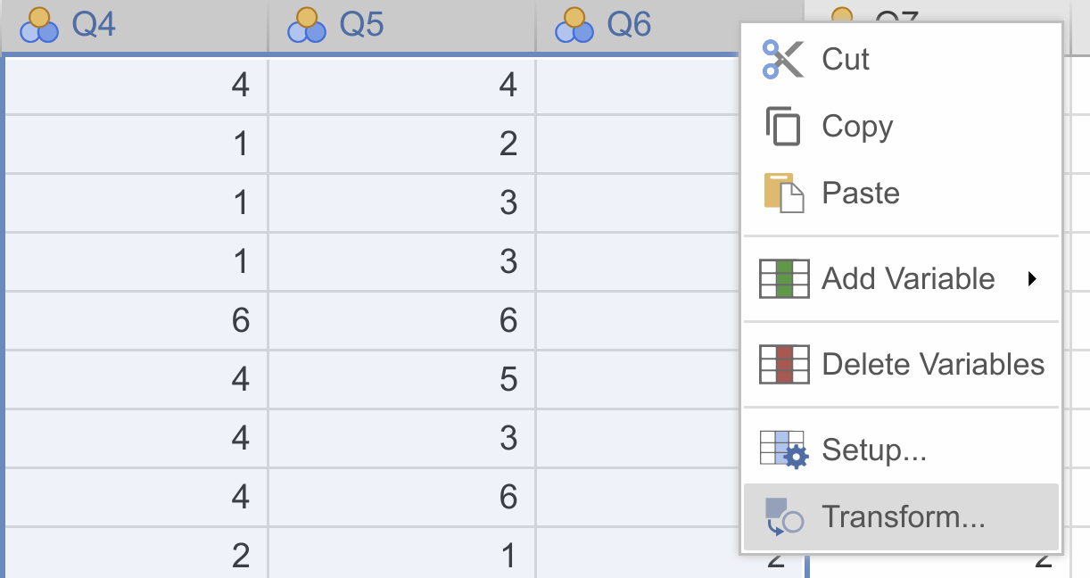Once selected, you can either select Transform from the data tab, or right click and choose Transform from the menu.

Either right-click on one of the selected variables, and click Transform...:

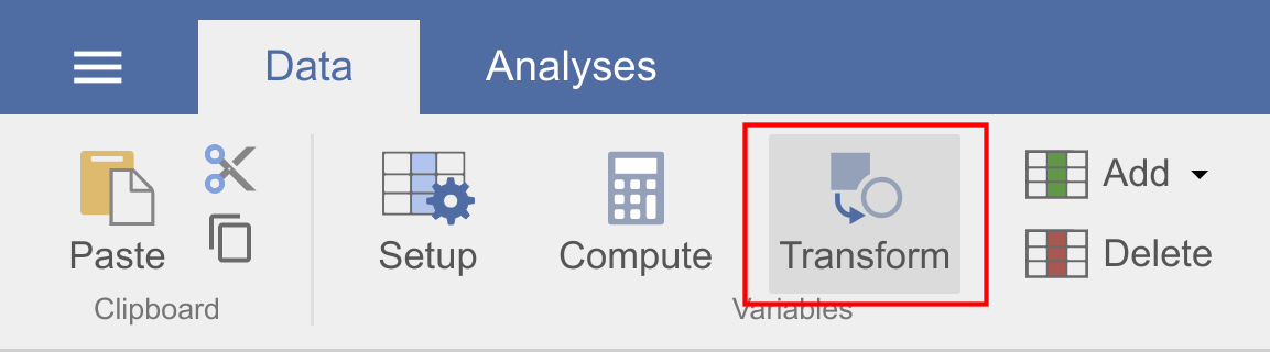
or head to the Data-ribbon, and click Transform:

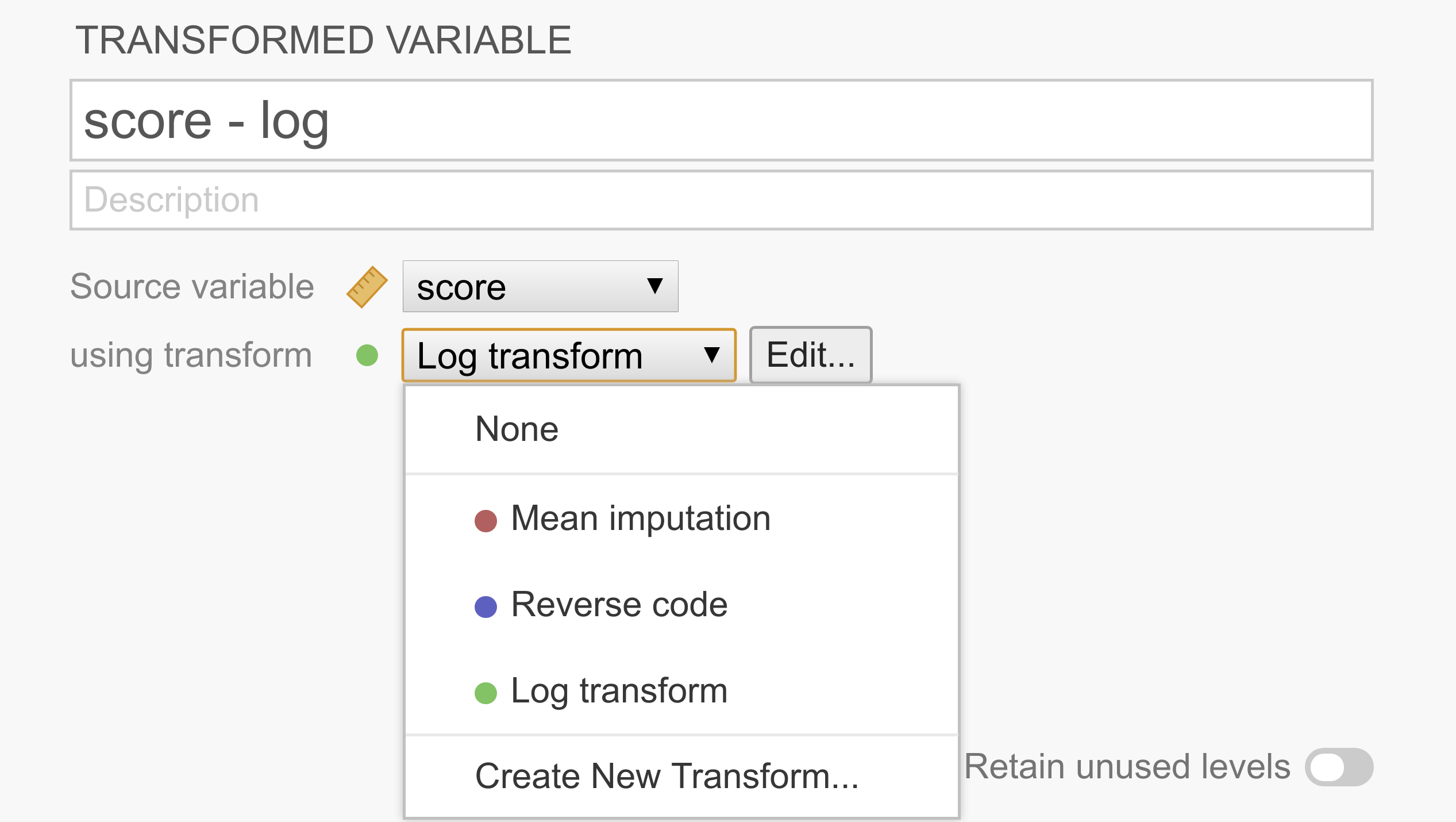
This constructs a second “transformed variable” for each column that was selected. In the following example, we only had a single variable selected, so we’re only setting up the transform for one variable (called score - log), but there’s no reason we can’t do more in one go.

As can be seen in the figure above, each transformed variable has a “source variable”, representing the original untransformed variable, and a transform, representing rules to transform the source variable into the transformed variable. After a transform has been created, it’s available from the list and can be shared easily across multiple transformed variables.

If you don’t yet have the appropriate transform defined, you can select Create new transform... from the list.

Create a new transformation

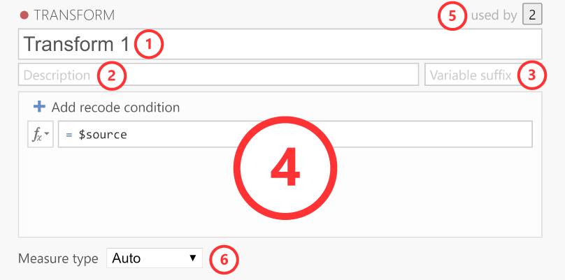
After clicking Create new transform... the transform editor slides into view:

The transform editor contains these elements.

1. Name: The name for the transformation.

2. Description: Space for you to provide a description of the transformation so you (and others) know what it does.

3. Variable suffix (optional): Here, you can define the default name formatting for the transformed variable. By default, the variable suffix will be appended to the source variable name with a dash (-) in between. However, you can override this behavior by using an three dots (…), which will be replaced by the variable name. For instance, if you transform a variable called Q1, you could use variable suffixes to apply the following naming schemes (if left empty, the transformation name is used as the variable suffix):

   log → Q1 - log ..._log → Q1_log log(...) → log(Q1)

4. Transformation: This section contains the rules and formulas for the transformation. You can use all the same functions that are available in computed variables, and to refer to the values in the source column (so you can transform them), you can use the special $source keyword. If you want to recode a variable into multiple groups, it’s easiest to use multiple conditions. To add additional conditions (i.e., if-statements), you click on the Add recode condition button:

5. Used by: Indicates how many variables are using this particular transformation. If you click on the number it will list these variables.

6. Measure type: By default the measure type is set to Auto, which will infer the measure type automatically from the transformation. However, if Auto doesn’t infer the measure type correctly, you can override it over here.

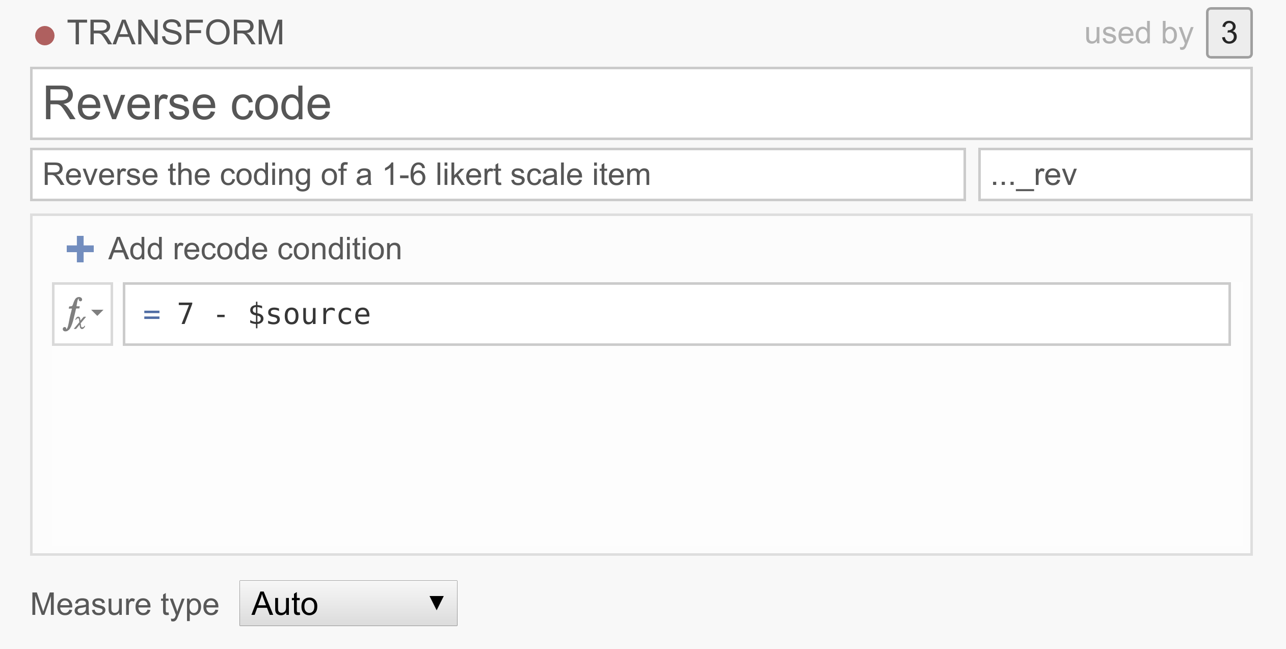
Example 1: Reverse scoring of items

Survey data often contains one or more items whose values need to be reversed before analyzing them. For example, we might be measuring extraversion with the questions “I like to go to parties”, “I love being around people”, and “I prefer to keep to myself”. Clearly a person responding 6 (strongly agree) to this last question shouldn’t be considered an extravert, and so 6 should be treated as 1, 5 as 2, 1 as 6, etc. To reverse score these items, we can just use the following simple transform:

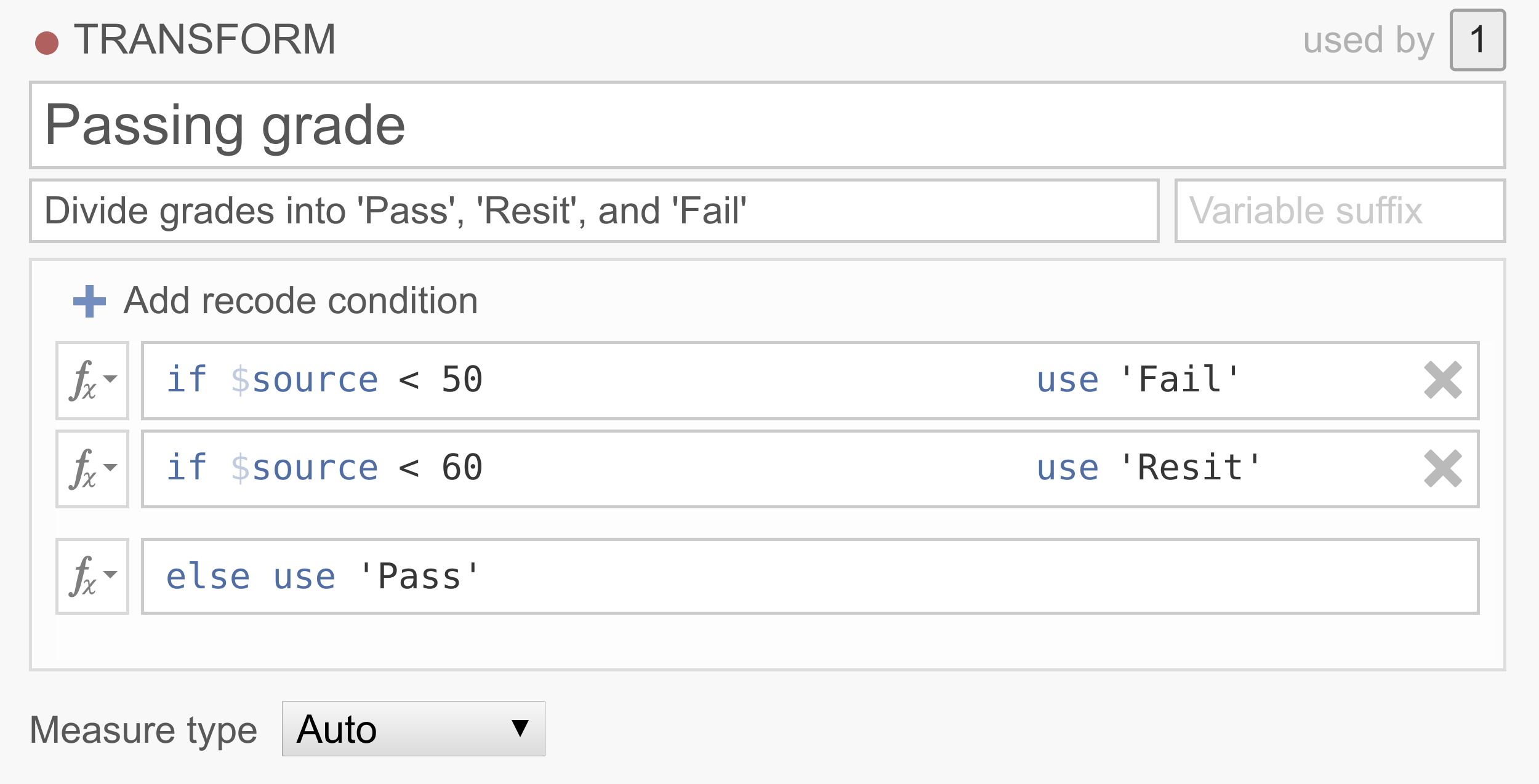
You can explore this transform by downloading <../_static/output/um_transform_ex1.omv> and opening the file transform_ex1 in jamovi.

Example 2: Recoding continuous variables into categories

In a lot of data sets people want to recode their continuous scores into categories. For example, we may want to classify people, based on their 0-100% test scores into one of three groups, Pass, Resit and Fail.

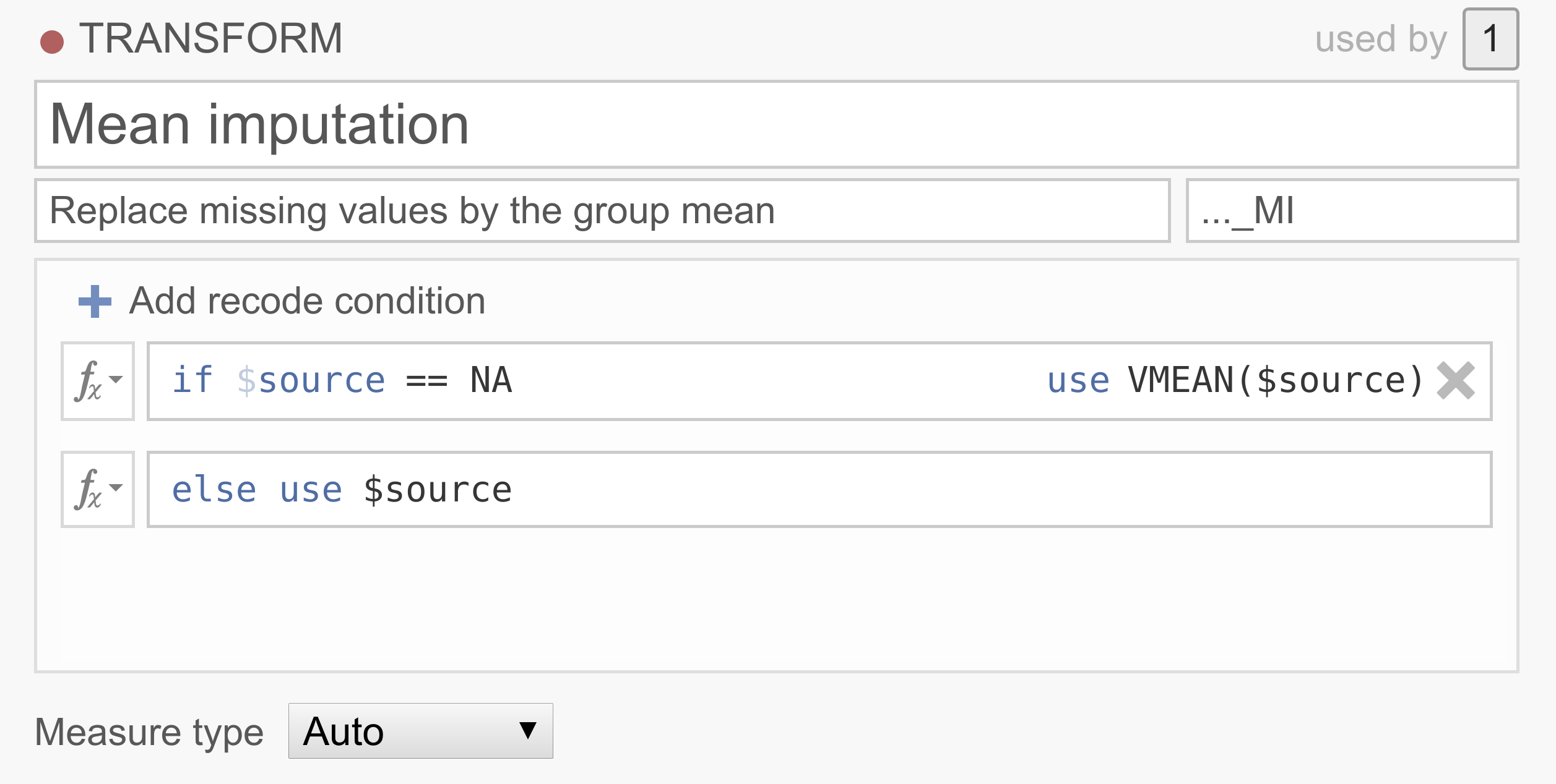
Note that the conditions are executed in order, and that only the first rule that matches the case is applied to that case. So this transformation basically says that if the source variable has a value below 50, the value will be Fail, if the source variable has a value between 50 and 60, the value will be Resit, and if the source variable has a value above 60, the value will be Pass. If you’d like an example data set to play around with, you can download <../_static/output/um_transform_ex2.omv> and use transform_ex2.omv.

Example 3: Replacing missing values

Now, let’s say your data set has a lot of missing values and removing the participants with missing values will end up in a severe loss of participants. There are a number of ways to deal with missing data, of which imputation is quite common. One pretty straightforward imputation method replaces the missing values with the variable mean (i.e., mean substitution). Although there are a bunch of problems associated with mean substitution and you should probably never do it, it does make for a neat demonstration…

Note that jamovi has borrowed NA from R to denote missing values. Don’t have a good data set handy? You can try it out yourself by downloading <../_static/output/um_transform_ex3.omv> and opening the transform_ex3.omv data set.

Filter

Mit Filtern können Sie in jamovi Zeilen herausfiltern, die Sie aus Ihrer Analyse ausschließen wollen. Zum Beispiel können Sie die Umfrageantworten von Personen nur dann einbeziehen, wenn diese ausdrücklich der Verwendung ihrer Daten zugestimmt haben, Sie könnten alle Linkshänder ausschließen, oder Personen, die bei einer experimentellen Aufgabe „unter Zufallsniveau“ abschneiden. Filter eignen sich auch, um extreme Werte auszuschließen, zum Beispiel solche, die mehr als 3 Standardabweichungen vom Mittelwert abweichen oder die Extremwerte in Bezug auf ihren Interquartilbereich sind (IQR; d.h. Extremwerte außerhalb der Whisker im Box-Whisker-Diagramm).

Die Filter in jamovi bauen auf dem jamovis‘ Formelsystem für Berechnete Variablen auf. Dies ermöglicht das Erstellen (und Filtern) beliebig komplexer Formeln.

Row filters

jamovi filters are demonstrated using the Tooth Growth data set which is included with jamovi (☰ → Open → Data Library). Select the Filters button from the Data ribbon. This opens the filter view and creates a new filter called Filter 1.

In the short video, we specify a filter to exclude the 9th row. Perhaps we know that the 9th participant was someone just testing the survey system, and not a proper participant (Tooth Growth is actually about the length of guinea pig teeth, so perhaps we know that the 9th participant was a rabbit). We can simply exclude them with the formula:

ROW() != 9

In this expression the != means ‘does not equal’. If you’ve ever used a programming language like R this should be very familiar. Filters in jamovi exclude the rows for which the formula is not true. in this case, the expression ROW() != 9 is true for all rows except the 9th row. When we apply this filter, the tick in the Filter 1 column of the 9th row changes to a cross, and the whole row greys out. If we were to run an analysis now, it would run as though the 9th row wasn’t there. Similarly, if we already had run some analyses, they would re-run and the results would update to values not using the 9th row.

Typically, we would like to have more complex filters than this! The Tooth Growth example contains the length of teeth from guinea pigs (the len column) fed different dosages (the dose column) of supplements: vitamin C or orange juice (recorded in the supp column as VC and OJ). Let’s assume that we’re interested in the effect of dosage on tooth length. We might run an ANOVA with len as the dependent variable, and dose as the grouping variable. But let’s say that we’re only interested in the effects of vitamin C, and not of orange juice. Then, we can use the formula:

supp == 'VC'

In fact we can specify this formula in addition to the ROW() != 9 formula if we like. We can add it as another expression to Filter 1 (by clicking the small + beside the first formula), or we can add it as an additional filter (by selecting the large + to the left of the filters dialog box). As we’ll see, adding an expression to an existing filter does not provide exactly the same behaviour as creating a separate filter. In this case however, it doesn’t make a difference, so we’ll just add it to the existing filter. This additional expression comes to be represented with its own column as well, and by looking at the ticks and crosses, we can see which filter or expression is responsible for excluding each row.

But let’s say we want to exclude from the analysis all the tooth lengths that were more than 1.5 standard deviations from the mean. To do this, we’d take a z-score, and check that it falls between -1.5 and 1.5. we could use one of the following formulas (this second formula is a great way to demonstrate to students what a z-score is):

-1.5 < Z(len) < 1.5
-1.5 < (len - VMEAN(len)) / VSTDEV(len) < 1.5

There are a lot of functions available in jamovi, and you can see them by clicking the small f_x beside the formula box.

Now let’s add this z-score formula to a separate filter by clicking the large + to the left of the filters, and adding it to Filter 2.

With multiple filters, the filtered rows cascade from one filter into the next. So only the rows allowed through by Filter 1 are used in the calculations for Filter 2. In this case, the mean and standard deviation for the z-score will be based only on the vitamin C rows (and also not on row 9). In contrast, if we’d specified our Z() filter as an additional expression in Filter 1, then the mean and standard deviation for the z-score would be based on the entire dataset. In this way you can specify arbitrarily complex rules for when a row should be included in analyses or not (but you should pre-register your rules).[1]

Column filters

Whereas row filters are applied to the data set as a whole, sometimes you want to just filter individual columns. Column filters come in handy when you want to filter some rows for some analyses, but not for all. This is achieved with the computed variable system. With the computed variables we create a copy of an existing column, but with the unwanted values excluded.

In the Tooth Growth example, we might want to analyse the doses of 500 and 1000, and 1000 and 2000 separately. To do this we create a new column for each subset. So in our example, we can select the dose column in the jamovi spreadsheet, and then select the Compute button from the data tab. This creates a new column to the right called dose (2), and same as the filters, we can enter a formula. in this case we’ll enter one of the formulas below (the do the same, the second is perhaps easier to understand):

FILTER(dose, dose <= 1000)
FILTER(dose, dose == 1000 or dose == 500)

The first argument to the FILTER() function (in this example dose) is what values to use in the computed column. The second argument is the condition; when this condition isn’t satisfied, the value comes across blank (or as a “missing value” if you prefer). So with this formula, the dose (2) column contains all the 500 and 1000 values, but the 2000 values are not there.

We might also change the name of the column to something more descriptive, like dose 5,10. Similarly we can create a column dose 10,20 with the formula FILTER(dose, dose != 500). Now we can run two separate ANOVAs (or t-tests) using len as the dependent variable, and dose 5,10 as one grouping variable in the first analysis, and dose 10,20 in the other. In this way we can use different filters for different analyses. Contrast this with row filters which are applied to all the analyses.

It may also have occurred to you, that with FILTER() we can do what might be called a “poor man’s split variables”: You can create splits using FILTER(). For example, we could split len into two new columns len_VC and len_OJ with the functions FILTER(len, supp == 'VC') and FILTER(len, supp == 'OJ') respectively. This results in two separate columns which can be analysed side-by-side.

[1]	Pre-registration is a solution to p-hacking, not deliberately making software difficult to use! Don’t p-hacking. Your p-hacking harms more people than you may assume.